EEC 193A Lab 1 Part 2: Lane Line Detection

In this project, you will work in groups of 3 to write a software pipeline using traditional computer vision techniques in C++ to identify the lane boundaries in a video and use those lane boundaries to output waypoints that a self-driving car would follow. This project will also give you initial exposure to the following software tools, libraries, and concepts: Git, Docker, CMake, OpenCV, Boost, and Smart Pointers. However, all the aforementioned are simply tools to help you develop a working lane line detection pipeline. They are not the main focus of this project. The main focus is to ensure you understand the general steps of the lane line detection algorithm and how to implement those steps at a high-level.

The main component of this lab will be OpenCV. We will be using OpenCV 3.4.4. Throughout this assignment, you may find it useful to refer to the offical OpenCV documentation: opencv-docs

General Information

Deadline: 06:09 pm, Saturday, January 19th, 2019

For every 24 hours your submission is late, 5% will be deducted from your total score.

Setting up the Environment

Your environment will be contained in a docker container. You will need to create your container from the eec193_lab1 docker image which is already on the two GPU servers dedicated to this course: atlas.ece.ucdavis.edu and kronos.ece.ucdavis.edu. However, you do not have to do your work remotely on the provided servers. We also provide a Dockerfile if you would like to do this project on your own machine using your favorite text editor.

SSH into the machines using the following commands:

# for atlas.ece.ucdavis.edu
ssh -Y kerberos_id@atlas.ece.ucdavis.edu

# for kronos.ece.ucdavis.edu
ssh -Y kerberos_id@kronos.ece.ucdavis.edu

Or if you'd like to work on your host machine, first make sure you download docker community edition for your operating system: docker-ce

Then download this Dockerfile, make sure you are in the same directory as the Dockerfile, and run the following command:

docker build -t eec193_lab1 .

This may take anywhere from 5-60 minutes depending on your internet speed. Once completed, verify the image eec193_lab1 exists by running the following command:

docker images

Once you are on a machine with the eec193_lab1 image, run the following command to mount your container:

docker run -it --name=lanelines -v <any_path_on_host_machine>:/root/eec193_lab1 eec193_lab1

The --name flag creates a docker container named "lanelines" which will be your project environment.

The -v flag mounts a shared volume between your docker container and host machine. This will allow you to modify code files in your docker container from your host machine. It is highly recommended that when you choose the folder on your host machine that the folder is empty so that your project folder isn't full of unnecessary clutter.

Whenever you wish to enter your docker container again, make sure it is running by running the command:

docker container ls

If you don't see the container "lanelines", then you need to start it by running the following command:

docker start lanelines

Enter your docker container by running this command

docker exec -it -e DISPLAY=<IPv4_Address>:0.0 lanelines /bin/bash

The -e flag passes an environment variable, which in this case is your DISPLAY variable. This is to forward your display port so you can view images from your docker container. You can find your IPv4_Address by typing ifconfig.

Once inside your docker container, change to the appropriate directory.

cd /root/eec193_lab1

The Pipeline

Before going into lower-level details of each step of the lane line detection, we will first give a summary of every step in the pipeline.

• Compute the camera calibration matrix and distortion coefficients given a set of chessboard images.
• Apply a distortion correction to the raw input images.
• Apply a perspective transform to transform the image into a "birds-eye view."
• Use color and gradient thresholds to isolate the lane line pixels, creating a binary image.
• Cluster the lane lines into their individual instances using the window search algorithm
• Find the polynomial best-fit lines for each lane line
• Use the best-fit lines to generate waypoints
• (Optional) Calculate other potentially helpful information such as center offset, radii of curvature, etc.
• (Optional) Use history information to smooth the best-fit lines across frames, such as using a simple-moving average or other filtering techniques
• Warp the detected lane boundaries and waypoints back onto the original image.
• Output visual display of the lane boundaries and waypoints

Phase 1: Camera Calibration

This project is broken into two CMake projects. The first of which is the camera calibration. You may find this project at camera_calibration/. You will be modifying src/calibrate_camera.cpp and src/intrinsics_tester.cpp.

In order to accurately measure distance from images, we must first correct any distortions caused by the lens of the camera. This is done by taking pictures of a well-defined, high-contrast object at different angles: a checkerboard. Using a set of checkerboard images, we can obtain a camera matrix and list of distortion coefficients which can be used to undistort images from a particular camera.

We have provided you with two sets of checkerboard images from two different cameras. One is a set of checkerboard images provided by Udacity which are located at camera_calibration/camera_cal/. The other set was taken at UC Davis which is located at camera_calibration/calibration_images/. We would like you to find the camera matrix and list of distortion coefficients for both cameras.

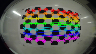
Finish all the TODOs in camera_calibration/src/calibrate_camera.cpp to find the camera matrix and distortion coefficients, which will then be saved to a yaml file. Be sure you are saving the drawn chessboard corners images to camera_calibration/drawn_corners/. To help verify everything was done correctly, there should be at least 20 images in that folder with checkerboard corners drawn. The drawn corners will look like something like the below picture.

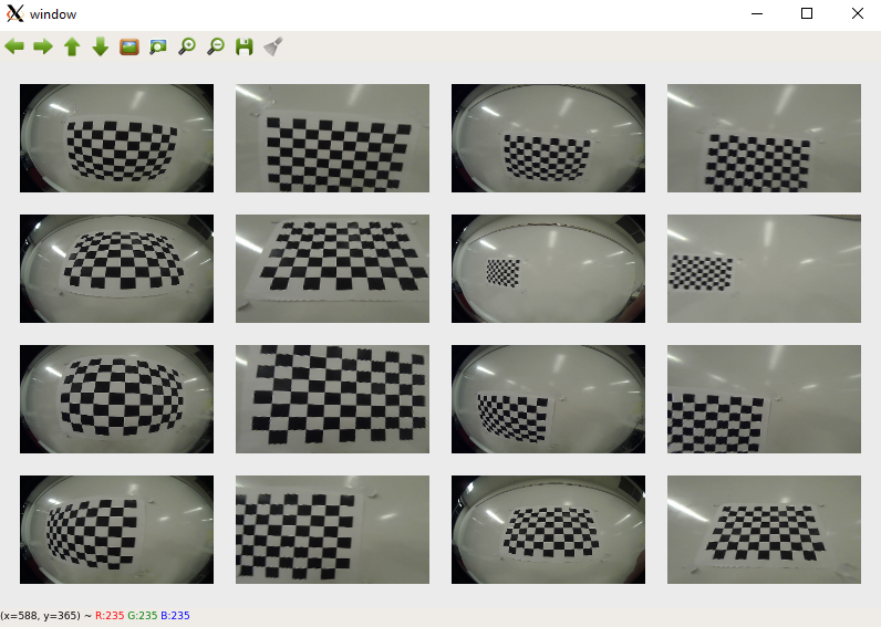
To finally verify your camera calibration, finish src/intrinsics_tester.cpp. All you need to do is use your camera matrix and list of distortion coefficients saved in your yaml file to undistort any 8 checkerboard images and visually verify they are undistorted. Be sure to show the distorted and undistorted images side-by-side.

If you are undistorting the images provided by the UC Davis camera, your results should look similar to this:

The functions you will need for this part are cv::cvtColor, cv::findChessboardCorners, cv::drawChessboardCorners, cv::calibrateCamera, cv::undistort.

Basic Build Instructions

These instructions should be followed from the top project directory.

1. cd camera_calibration
2. Make a build directory: mkdir build
3. Move to build directory: cd build
4. Generate Makefile: cmake ..
5. Build project: make

Running the executables

This will generate the executables calibrate_camera, and instrinsics_tester.

To run the first executable:

./calibrate_camera <path_to_yaml_file> <path_to_checkerboard_images>\*.png

To run the second executable:

./intrinsics_tester <path_to_yaml_file> <path_to_checkerboard_images>\*.png

NOTE: you may have to change the extension to *.jpg if the images are JPEG.

Your yaml files should be saved in the top directory. For the Udacity camera, name the yaml file udacity_parameters.yaml. For the UC Davis camera, name the yaml file fisheye_parameters.yaml.

Phase 2: Lane Line Detection

This is the real lane line detection project. It is another CMake project that is located at lane_line_detection/.

This project is purposefully broken into many subparts. Most of them with their own module file and tester file. This is to both ensure you build your program incrementally and to allow you to parallelize your work.

Throughout this project, you will be working with the same 8 test images located at images/test_images/ until you have built the full pipeline. Once you are satisfied with how your lane line detection is behaving on the 8 test images, you will run your pipeline on a test video.

Phase 2.1 Perspective Transformation

To more easily isolate the lane line pixels, it helps to get a birds-eye view of the road, so we cut out unnecessary information. You will do that by performing a perspective transformation.

This is done by defining four source points which define your ground plane and four destination points which define where your ground plane will appear in the birds-eye view.

You will be modifying perspective_transform_tester.cpp to apply the perspective transformation to 8 test images provided at images/test_images/.

The goals of this part are as follows:

• Tune the source and destination points appropriately to get an accurate birds-eye view
• Save the final birds-eye view images to images/warped_images/ for use in the next part

Your source and destination points will be in the yaml file. This is so you don't have to re-compile every time you wish to modify your source and destination points.

Copy and paste the following to the bottom of udacity_parameters.yaml.

# Order: bottom left, top left, top right, bottom right
source points: [ 0., 400.,
                 300., 720.,
                 900., 720.,
                 720., 400. ]

# Order: bottom left, top left, top right, bottom right
destination points: [ 100., 0.,
                      100., 600.,
                      1000., 600.,
                      1000., 0. ]

The source and destination points are not correct. You will have to adjust them yourself. You are provided with a helper function draw_viewing_window to help you visualize your source and destination points. Below is an example of how to use it:

// draw green source points on your source image with thickness of 5
draw_viewing_window(src_img, src_points, cv::Scalar(0,255,0), 5);

When applying the perspective transformation, be sure you are first undistorting the image using cv::undistort!! If you do not have the camera matrix and distortion coefficients yet, you can still do this part of the lab without undistorting the images, but be sure to come back and undistort the images when you do get the camera matrix and distortion coefficients.

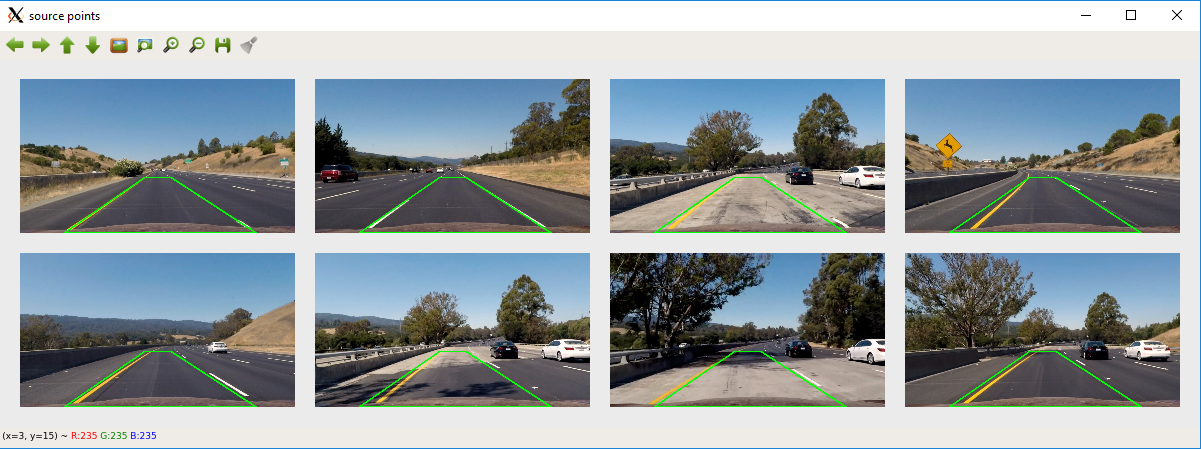
Your source points should define your ground plane. Use an image with straight lane lines to help you do this. Your source points should draw out a trapezoid . Be sure to visually verify they are what you expect.

Here's an example:

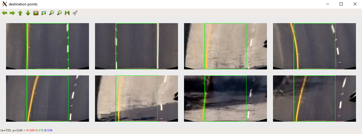
Your destination points should define a rectangle located at the bottom of the image. The smaller the area of this rectangle, the more zoomed out your birds-eye view will be. The larger the area, the more zoomed in you will be.

Use your source and destination points to obtain the perspective transform matrix using cv::getPerspectiveTransform. Then apply the perspective transformation on the 8 test images using cv::warpPerspective.

Here's roughly what your drawn destination points should look like. However, your destination points do not need to be exactly the same. It's up to you to decide your own magnification factor.

Basic Build Instructions

These instructions should be followed from the top project directory.

1. cd lane_line_detection
2. Make a build directory: mkdir build
3. Move to build directory: cd build
4. Generate Makefile: cmake ..
5. Build project: make

Running the executable

This will generate many executables. However, for this part, you only need to worry about perspective_transform_tester.

To run the executable:

./perspective_transform_tester <path_to_yaml_file> <path_to_test_images>\*.png

NOTE: you may have to change the extension to *.jpg if the images are JPEG.

When you are satisfied with your birds-eye view, save the birds-eye-view images (without the drawn destination points) to images/warped_images/ using something like cv::imwrite, so you can use them for the next part.

Phase 2.2 Color and Gradient Thresholds

To properly isolate the lane line pixels, you will apply color and gradient thresholds.

If you have not finished Phase 2.1, then you may use the provided example warped images located at images/example_warped_images/ to cmplete this phase.

The files you'll be modifying for this part are src/thresholds.cpp, src/thresholds_tester.cpp, and include/thresholds_tester.hpp.

The goals of this part are as follows:

• Finish the function abs_sobel_thresh
• Finish the function sobel_mag_dir_thresh
• Write your own function, with an API you decide, apply_thresholds
• Save the final results to images/thresholded_images/

Throughout this part, it may be most efficient for you to complete one function, test it in src/thresholds_tester.cpp through visualization, make sure it looks correct, and do this for all three functions. However, when you finish defining apply_thresholds, your tester file should just be a for-loop that is using apply_thresholds on all your warped images, visualizing the results, and saving them.

Basic Build Instructions

These instructions should be followed from the top project directory.

1. cd lane_line_detection
2. Make a build directory: mkdir build
3. Move to build directory: cd build
4. Generate Makefile: cmake ..
5. Build project: make

Running the executable

This will generate many executables. However, for this part, you only need to worry about thresholds_tester.

Run this command to execute:

./thresholds_tester <path_to_warped_images>

Phase 2.2.1 abs_sobel_thresh

The function abs_sobel_thresh uses the Sobel algorithm to find the gradient of the image with respect to x or y, takes the absolute value of the gradient, and applies some upper and lower thresholds, returning some binary image.

Below are some example images with the corresponding function calls:

abs_sobel_thresh(warped_img, sobelx_img, 'x', 15, 40, 100);

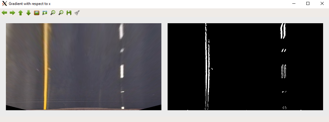
abs_sobel_thresh(warped_img, sobely_img, 'y', 15, 40, 100);

Your images do not need to look exactly the same given the same inputs. But they should be very similar.

The steps are as follows:

1. Find gradient with respect to x or y depending on input char orient
2. Take absolute value of gradient
3. Normalize all values to be between 0-255
4. Convert image to type CV_8U (8-bit unnsigned cv::Mat)
5. Apply thresholds

Be sure to normalize before converting the image to 8-bit unsigned ints, or else you will lose information, and it will be wrong!

When you do normalize, it's up to you, but you don't need to write a for-loop iterating through every pixel. It is easy to do pixel-wise math with cv::Mat.

Here's an example of performing pixel-wise multiplication and division:

img = 2*img/5;

Performing pixel-wise addition and subtraction is just as intuitive.

Some opencv functions you might find useful: cv::Sobel, cv::abs, cv::minMaxLoc, cv::Mat::convertTo, cv::threshold, cv::bitwise_and, cv::bitwise_or.

For the thresholding, you don't necessarily have to use opencv functions like cv::threshold. You could just do this:

img_thresholded = img > 20 & img < 100;

img is of type CV_8U with 1 channel. The resulting image will be a binary image of values 255 and 0. Any pixel values between 20 and 100 will be 255. The rest will be 0. You can use the | operator for logical or.

While there is no threshold range that will perfectly isolate the lane line pixels for all the images, try as best as you can to isolate the lane line pixels using abs_sobel_thresh.

Phase 2.2.2 sobel_mag_dir_thresh

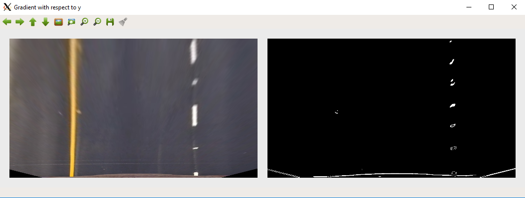
The function sobel_mag_dir_thresh uses the Sobel algorithm to find the magnitude and direction of the gradient of an image and applies some lower and upper thresholds. So there will be two output images.

Below are some example images with the corresponding function call:

sobel_mag_dir_thresh(warped_img, sobel_mag_img, sobel_dir_img, 15, 20, 100, 0.0, 0.2);

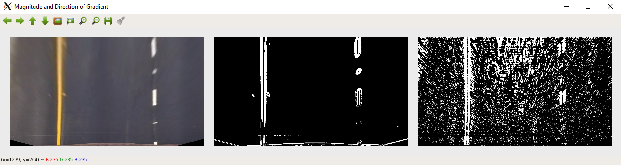
The middle image is the magnitude of the gradient after thresholds. The far-right image is the direction of the gradient after thresholds.

The steps are as follows:

1. Find both the gradient with respect to x and y
2. Take the absolute value of the gradient images
3. Calculate the magnitude and direction of the gradient
4. Normalize the magnitude of the gradient to be between 0-255
5. Convert the magnitude of the gradient to type CV_8U
6. Apply thresholds for both the magnitude and direction

Notice how we only need to normalize the magnitude of the gradient, not the direction of the gradient. This is because we are keeping the direction of the gradient as a floating type. The values will always be between 0 and pi/2 radians.

The OpenCV functions you'll need are the same as Phase 2.2.1, but you'll also need cv::cartToPolar to calculate the magnitude and direction.

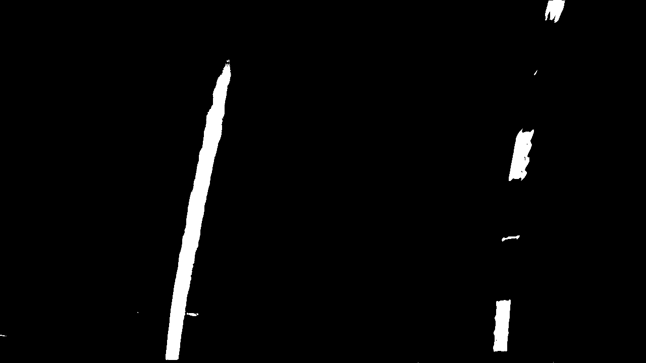
Once again, there is no threshold range that will perfectly isolate the lane line pixels, but you can do better by logically and-ing and or-ing the different gradient images.

Some examples:

You can try logically and-ing all your gradient images.

img_thresholded = gradx & grady & grad_mag & grad_dir;

You can try using a combination of logical and and logical or.

img_thresholded = (gradx & grady) | (grad_mag & grad_dir);

Try different things. You may find that some gradient thresholds are not as useful as others. You do not have to use all of them.

Phase 2.2.3 apply_thresholds

This is to ensure your code is modularized. apply_thresholds will wrap all the threshold functions you want to call into one function call. You may define the inputs and outputs however you want. The only requirement is that the input and output must be of type cv::Mat. You will need to define the function prototype in include/thresholds.hpp and the actual implementation in src/thresholds.cpp.

Other than applying your gradient thresholds, you also need to apply color thresholds in your apply_thresholds function. OpenCV makes this really easy with its cv::inRange function.

When trying to isolate the lane line pixels using colors, you will find that the RGB color model does not provide an easy way to do this. Instead, it is easier to isolate the lane line pixels using channels of images which are of a different color space. Some color spaces you may find useful are HLS and LAB. The L channels are generally good at extracting the white pixels, while the S and B channels are generally good at extracting the yellow pixels.

While not required, you may want to first view each of the channels individually to see for yourself which channels are most useful for extracting the lane line pixels. cv::extractChannel would be useful for that.

When you're done deciding on your color thresholds, you should decide how you want to logically and/or your gradient and color thresholded images, and make sure it is all wrapped inside the apply_thresholds function.

Example thresholded images are provided in images/example_thresholded_images/.

Phase 2.3 Defining a Lane Line Class

Before we move onto the window search, it will be useful to define a lane line class so our code will be more scalable. In this phase you will be modifying include/lane_line.hpp and src/lane_line.cpp.

I have included a lane line class definition in include/lane_line.hpp that is very similar to the one a TA used and is extremely bare bones. There is nothing in this lane line class that allows for using history information, which you may find important to incorporate once you are testing your algorithm on videos. You may also wish to add visualization methods to your lane line class, or they could be entirely separate functions. You will be provided with helpful visualization code in the next few phases. You may use this lane line class as a starting point or create your own. It is all up to you.

Be sure to also write the corresponding lane_line.cpp for the actual implementation of your lane line class. At bare minimum, implement a constructor. If you decide to keep the fit method, you may figure that part out later when you've clustered the lane line pixels with the window search.

You may use the following for the pixels to meters conversion factors:

xm_per_pix = 3.7/700.
ym_per_pix = 30./720.

Phase 2.4 Window Search

To cluster the lane lines, we will use window search. Window Search is a clustering algorithm particular to clustering lane lines. We need to be able to cluster the different instances of lane lines to find the best-fit lines.

In this phase, you will be modifying window_search.cpp and window_search_tester.cpp.

The goals are as follows:

• Use the window search algorithm to cluster the lane lines in the 8 test images
• Visualize the window search
• Compute the best-fit lines
• Visualize the best-fit lines
• Compute the waypoints in both pixels and meters
• Visualize the waypoints

Phase 2.4.1 Implementing the Window Search

The window search algorithm starts by looking at the column-wise histogram peaks on the left and right-hand side of the binary warped image, choosing the largest peaks for each side. The locations of these peaks are where the window searches will start.

Below is an example of the histogram for a particular binary warped image (not exactly to scale):

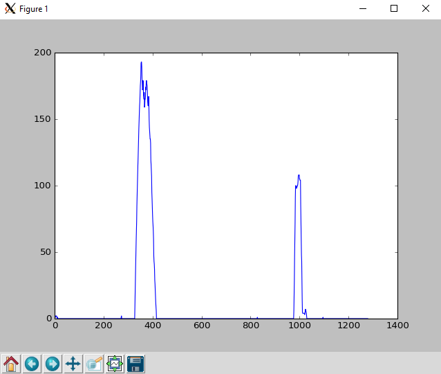
Once you've defined your starting position, the window search re-centers itself based on the mean position of the non-zero pixels inside the window until it reaches the boundaries of the image.

You may re-center based on both x and y position or only x position. Re-centering based only on x position is faster as this allows you to control the number of windows. However, for sharp curvature, re-centering based on both x and y position may become unavoidable. For this lab, you should only need to re-center based on x position.

The psuedo-code for the window search algorithm is as follows

n_windows = 9 # number of windows
margin = 100 # width/2 of the window
minpix = 75 # minimum number of pixels required to re-center window
x_current = getPeakBase() # starting x position of window search

for window in range(n_windows):

  Update top, bottom, left, and right sides of window

  drawRectangle() # draw the rectangle for debugging

  colorNonZero() # color in the non-zero pixels inside of window for debugging

  good_inds = findNonZero() # obtain list (cv::Mat) of non-zero pixel locations in window

  if good_inds is not None:

    good_inds_x = good_inds[:,:,0] # extract all x positions from first channel
    good_inds_y = good_inds[:,:,1] # extract all y positions from second channel

    line_inds_x.append(good_inds_x) # Push x values to list (cv::Mat) of all x values
    line_inds_y.append(good_inds_y) # Push y values to list (cv::Mat) of all y values

    if (len(good_inds) > minpix):
      x_current = mean(good_inds_x) # update x position of window

For visualizing the window search, you may find the code below useful:

// draw window green
cv::rectangle(window_img, cv::Point(win_left, win_bottom),
cv::Point(win_right, win_top), cv::Scalar(0,255,0), 2);

// color in pixels inside of window according to color of lane line
window_img(cv::Range(win_bottom,win_top),
cv::Range(win_left,win_right)).setTo(lane_lines[i]->color,
binary_warped(cv::Range(win_bottom,win_top),
cv::Range(win_left,win_right)) != 0);

Here's what your window search should look like this:

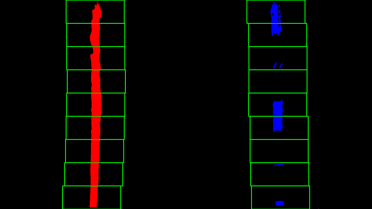
You need to call the window search for every lane line you are looking for, which in this case is two. This should all be wrapped nicely in the window_search function defintion provided to you in include/window_search.hpp and src_window_search.cpp.

NOTE: You are allowed to change the function definition for window_search. The only requirement is that it should take in a binary warped image and some list of pointers on lane lines as inputs and output a visualization of the window search. You don't have to use smart pointers on lane lines. You may use C-Style pointers. However, if you're going to use C++, you might as well use what C++ has to offer and not use C-Style pointers...

Phase 2.4.2 Calculating the Best-Fit Lines

Once you have finished window search for one lane line, you need to find the best-fit line for that lane line. Remember that the lane lines are functions of y, not x. You may use the linspace, polyfit, and polyval functions defined in include/signal_proc.hpp and src/signal_proc.cpp to help you with this. Use a second order-polynomial to fit the lane lines.

Here's an example:

// get best-fit coefficients of second-order polynomial
polyfit(line_inds_y, line_inds_x, best_fit, 2);

// generate y-values for plotting best-fit line
linspace(0, binary_warped.rows-1, binary_warped.rows, ploty);

// generate x values of best-fit line
polyval(ploty, fitx, best_fit);

Be sure to find the best-fit lines both in pixels and meters.

You will probably want to visualize the best-fit lines on both your window search image and on your original input image. This will require drawing best-fit lines on two images as shown below:

/*
 * NOTE:
 * In this context, left_line and right_line are not lane lines!
 * Instead, they define the left and right line boundaries of one lane line.
 * Also, margin is the margin variable used in the window search algorithm.
 */
cv::Mat pts1, pts2, left_line, right_line, poly_img;

// make left line boundary of lane line
std::vector<cv::Mat> left_merge = {fitx-margin, ploty};
cv::merge(left_merge, left_line);

// make right line boundary of lane line
std::vector<cv::Mat> right_merge = {fitx+margin, ploty};
cv::merge(right_merge, right_line);
cv::flip(right_line, right_line, 0);
cv::vconcat(left_line, right_line, pts2);
pts2.convertTo(pts2, CV_32S);
std::array<cv::Mat,1> poly = { pts2 };

// draw lane line as polygon
poly_img = cv::Mat::zeros(window_img.rows, window_img.cols, window_img.type());
cv::fillPoly(poly_img, poly, cv::Scalar(0,255,0));
cv::hconcat(fitx, ploty, pts1);
pts1.convertTo(pts1, CV_32S);

// draw thin best-fit line on image with window search
cv::polylines(window_img, pts1, 0, cv::Scalar(0,255,255), thickness1);
cv::addWeighted(window_img, 1.0, poly_img, 0.3, 0.0, window_img);

// draw thick best-fit line on blank image to be warped back for final result
cv::polylines(final_result_img, pts1, 0, color, thickness2);

Your results will look something like this:

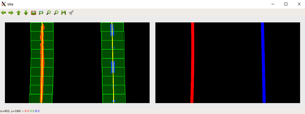
Don't move on until you are able to generate the images above for all 8 test images. Notice how the right image shows the best-fit lines on a black image. This is technically ready to be warped back into the original view, so we can try our pipeline on a video. But we first need to generate some waypoints in between those best-fit lines.

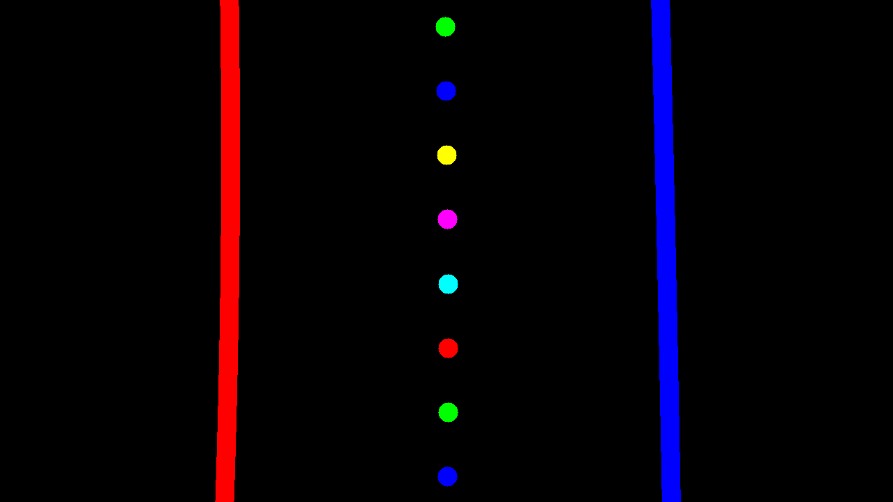
Phase 2.4.2 Generating Waypoints

Now that we have our left and right best-fit lines, we can generate waypoints along the center-line. Not only do we need to visualize the waypoints, we need to convert them to the proper frame of reference. While the waypoints in pixels will have their origin at the top left corner of the image, as is standard in computer vision, the waypoints in meters you will also be calculating will have their origin at the bottom-center of the image.

Complete the function generate_waypoints defined in include/window_search.hpp and src/window_search.cpp. The waypoints must be linearly spaced.

NOTE: You are allowed to change the function definition for generate_waypoints. The only requirements are that the inputs are the overlay image (far right image shown in last picture above) for visualizing waypoints, some list to pointers on lane lines (doesn't have to be smart pointers), the number of waypoints, and some way of initializing where to start and stop the waypoints. In the function definition given, this is done by specifying the top and bottom fractions of the image to start and stop the waypoints, which makes sense in this context because input image sizes can change. The output type must also NOT change.

You may visualize your waypoints by using cv::circle.

Here is an example of what your waypoint generation should look like if you generate 8 waypoints within the middle 90% of the image:

Phase 2.5 Putting it all Together

Congratulations! You've made every part of the lane line detection pipeline. Now it's time for you to put everything together. There are two main files for this project: images_main.cpp and video_main.cpp. As the names suggest, one is for testing your full pipeline on individual images that you select. The other one is for testing your full pipeline on video.

There is no starter code for this other than including headers.

For warping this image back into the original image space, simply switch the order of your source and destination points when calling cv::getPerspectiveTranform to generate some inverse perspective transformation matrix Minv. You can use this matrix to warp the perspective back. Then use cv::addWeighted to overlay that image back onto the undistorted input image. This is required.

The only other requirement is that your lane line detection output 8 clearly visible waypoints.

First put your pipeline together and ensure it works on the 8 test images in images_main.cpp.

Then write video_main.cpp to test your full pipeline on video. If I were you, I'd wrap the entire pipeline into one function to make it portable, but it's not required. The video is located at videos/project_video.mp4, and you may find an example output video at videos/example_output.mp4. Make sure to save your final output video in the videos/ folder.

For generating video, you may find this tutorial helpful: learn-opencv

If you find your lane line detection is failing on certain frames in the video, you can use cv::putText to put the frame number on your video, so that you can extract the failure frames to debug in images_main.cpp.

Submission

You will be submitting your entire project as a zip file on canvas. Only one person per group needs to submit. It is up to you whether or not to include the sandbox folder. Nothing in there will be graded.

Other than all the code files with the completed TODOs/function definitions and your final output video, make sure to include an AUTHORS in the top project directory eec193_lab1/ which contains the student ids of all the group members.

For example:

$ cat AUTHORS
000010001
000010002
000010003
$